As the title promises, I have spent some time for recapitulating the amplitude modulation and several reconstruction techniques. Today amplitude modulation isn’t very common, but was used for varoius applications like audio or signal transmissions in general.
Math
The amplitude modulation uses a high frequency signal $U_{C}$ which carriers the low frequency signal $U_{NF}$ into a higher frequency band.
$$ \begin{aligned} U_{NF} &= \hat{U}_{T} + \hat{U}_{NF} \cdot cos\left( \omega t \right)\\ U_{C} &= \hat{U}_{C} \cdot cos \left( \Omega t \right) \end{aligned}$$
For mathematical description, we choose \(\hat{U}_{C}\) to be \(1\) and we will end up.
$$ \begin{aligned} U_{AM} &= U_{NF} \cdot U_{C} \\ &= \left( \hat{U}_{T} + \hat{U}_{NF} cos\left( \omega t \right) \right) \cdot cos \left( \Omega t \right) \\ &= \hat{U}_{T} \cdot cos \left( \Omega t \right) + \frac{\hat{U}_{NF}}{2}\left( cos \left( \left( \Omega - \omega \right) \right) + cos \left( \left( \Omega + \omega \right) \right) \right) \end{aligned}$$
The last equation shows clearly the circumstance of three existing signals. The first one describes the DC1 component of the used low frequency signal, but with carrier frequency. The remaining two parts describing the produced sideband signals. They have the half amplitude of the low frequency signal and are positioned around the carrier frequency. For this script I demodulate the transmitted signal by using the convolution theory. Insted of use an envelope detector, it is also possible to multiply the time series of the carrier function again. Multiplication in the time domain will occur an convolution of booth signals in the frequency domain and as the low frequency part is shifted to higher frequencies, there will be existe multiple copies of the same alogn the frequency axis.
Python implementation
Import packages and libs
At first we will iport the needed packages. As you can see, I used matplotlib, numpy and scipy for this script. RaisedCos and Noisgen are selfwritten classes for signal generation.
import matplotlib.pyplot as plt
import numpy as np
import scipy as sp
import scipy.signal

from raised_cos import RaisedCos, Noisegen
Define constants
The constant values for this script are described below. I used a carrier frequency of 33 kHz and a signal frequency of 5.5 kHz for the lower signal part. The whole script uses a sample frequency of 1 MHz, so we get a sample period of 100 ns. ffc describes the cutoff frequency of the used reconstruction/low-pass filter and N is the number of used filter coefficients.
fc = 33e3                   # 33 kHz carrier
fs = 5.5e3                  # 5.5 kHz signal
fa = 1e7                    # sample frequency
dt = 1/fa                   # time resolution
ffc= 1.5*fs/fa              # cutoff frequency fir
N  = 150                    # filter order
Generate Signals and filter coefficients
For source signal generation I implemented the raised cosine function in Python. These function provides the possibility of a controllable bandwidth. The bandwidth may be modified by increasing the order \(N\). $$ \begin{aligned} U_{RC, N}\left( t\right) &= \frac{\left( -1 \right)^N}{2} \left(1 - cos\left( \frac{\omega t}{N} - \phi \right) \right) \cdot cos \left( \frac{\omega}{2} t - \phi\right) \end{aligned}$$

The Figure above shows the generated signal in time and frequency domain without noisefloor for different orders. As you can see the bandwidth is decreasing while the order was increased. For this example I used the sixth order, but neverless to say any other order would be also suitable.
Points = int(round(20e-4/dt))
# filter coefficients
h = sp.signal.firwin(numtaps=N, cutoff=fc, nyq=fa/2)
# time vector
x = np.arange(0,20e-4,dt)
ulf = np.zeros(Points)
# noise floor
noise = Noisegen( Points, 40)
#Points = int(round(4e-4/dt + 1))
# ultrasonic impulse
r = RaisedCos(6, Points, dt, 0, fs )
ulf = r.signal
#ulf = np.sin(2*np.pi*fs*x)
ulf += noise.signal
# thermal signal carrier
ucr = np.sin(2*np.pi*2*fc*x)
# carrier multiplied with low frequency signal
uam = ucr*ulf
# demodulate signal by mupltiplying the amplitude modulated signal again
ud = uam * ucr
# applyng the lowpass filter
r = sp.signal.lfilter(h, 1.0, ud )
# Scaling the amplitude
y  = 2*r
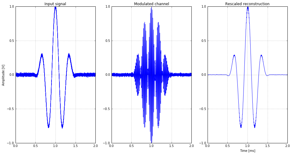
Plotting the signals
# plotting
f, axarr = plt.subplots(1, 3)
f.set_size_inches(16, 8)
axarr[0].plot(x*1e3, ulf)
axarr[0].set_title('Input signal')
axarr[0].set_ylabel('Amplitude [V]')
axarr[0].set_xlim([0, 2])
axarr[0].set_ylim([-1, 1])
axarr[0].grid()
axarr[1].plot(x*1e3, uam)
axarr[1].set_title('Modulated channel')
axarr[1].set_xlim([0, 2])
axarr[1].set_ylim([-1, 1])
axarr[1].grid()
axarr[2].plot(x*1e3, y)
axarr[2].set_title('Rescaled reconstruction')
axarr[2].set_xlabel('Time [ms]')
axarr[2].set_xlim([0, 2])
axarr[2].set_ylim([-1, 1])
axarr[2].grid()

plt.savefig('signals.png',dpi=150)
Direct current ↩︎