CFD simulations using Scientific Python

Introduction Link to heading

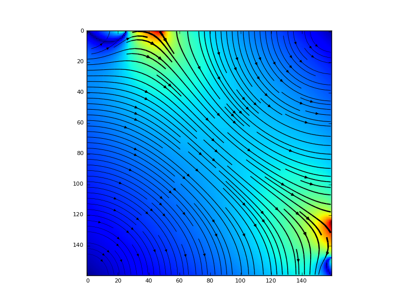
For some simulation topics of my Ph.D., I had to learn/recapitulate some basics about simulations techniques and fluid simulations. The original procedure and code could be found at Archer (UK National Supercomputing Service). This is a simple example for applying the finite difference approach to determine the flow pattern (CFD¹) in a cavity. For simplicity, we’re assuming a perfect liquid without viscosity, which also implies that there’re no vortices. The \(z\)-dimension of this setup was defined to be endless. We are interested in the directional velocity of the fluid.

A bit of math Link to heading

Finite Difference Method Link to heading

First order PDE Link to heading

For solving a first or higher order PDE² several methods exist. The easiest one is the finite difference method. For that method we’re needing a suitable approximation for the first derivative, for example the left aligned or forward difference:

$$ \frac{\partial}{\partial x} F \approx \frac{F(x + \Delta x) - F(x)}{\Delta x} + \mathcal{O(\Delta x)} $$

Also possible, the right aligned or backward difference:

$$ \frac{\partial}{\partial x} F \approx \frac{F(x) - F(x - \Delta x)}{\Delta x} + \mathcal{O(\Delta x)} $$

For a better approximation, we could also use the combination of forward and backward difference. This method is called the centered difference and is able to describe the derivative on position \(x\) only with knowledge about the neighbors left and right.

$$ \frac{\partial}{\partial x} F \approx \frac{F(x + \Delta x) - F(x - \Delta x)}{2\Delta x} + \mathcal{O(\Delta x)} $$

Second and higher order PDE Link to heading

$$ \begin{align} \frac{\partial^2 F}{\partial x^2} & = \frac{\partial } {\partial x} \left( \frac{\partial F}{\partial x}\right) \\ & \approx \frac{1}{\Delta x}\left(\frac{\partial F(x + \Delta x)}{\partial x} - \frac{\partial F(x - \Delta x)}{\partial x} \right) \\ & \approx \frac{1}{ \Delta x} \left( \frac{F(x+\Delta x) - F(x)}{ \Delta x} - \frac{F(x) - F(x - \Delta x)}{ \Delta x} \right)+ \mathcal{O}(\Delta x)^2 \\ & \approx \frac{1}{(\Delta x)^2} \Bigg( F(x + \Delta x) - 2F(x) + F(x - \Delta x) \Bigg) + \mathcal{O}(\Delta x)^2 \end{align} $$

Cavity problem solving Link to heading

For the given problem the following second-order PDE exist for the fluid flow \(\Psi\) which neglecting the existence of viscosity and toroids.

$$\frac{\partial^2 \Psi}{\partial x^2} + \frac{\partial^2 \Psi}{\partial y^2} = 0$$

Using the finite difference approach for second order PDEs we could rewrite the equation, which fully satisfies our problem.

$$ \begin{align} \frac{\partial^2 \Psi}{\partial x^2} + \frac{\partial^2 \Psi}{\partial y^2} & \approx \frac{1}{(\Delta x)^2} \Bigg( \Psi(x + \Delta x, y ) - 2 \Psi (x, y) + \Psi (x - \Delta x, y) \Bigg)\\ & + \frac{1}{(\Delta y)^2} \Bigg( \Psi(x, y + \Delta y) - 2 \Psi(x,y) + \Psi(x, y - \Delta y) \Bigg) \end{align} $$

For discretization we replace the continous terms \(x\) and \(y\) by their discrete replacements \(i\) and \(j\) and set the spatial resolution in \(x\)- and \(y\)-direction to \(1\) (\(\Delta x=\Delta y=1\) ).

$$ \frac{\partial^2 \Psi}{\partial x^2} + \frac{\partial^2 \Psi}{\partial y^2} \approx \Psi_{i+1,j} + \Psi_{i-1, j} + \Psi_{i,j-1} + \Psi_{i, j+1} - 4\cdot\Psi_{i,j} = 0 $$

With this approximation and the usage of the Dirchlet boundary condition (borders without sources are set to \(0\)) we could solve our problem. For velocity field \( \vec{u} \) computation, we calculate the partial differentiations.

$$ u_x (x,y) = \frac{\partial\Psi}{\partial y} = \frac{1}{2} \left( \Psi_{i,j+1} - \Psi_{i,j-1} \right)$$

$$ u_y (x,y) = \frac{\partial\Psi}{\partial x} = \frac{1}{2} \left( \Psi_{i+1,j} - \Psi_{i-1,j} \right) $$

Implementation Link to heading

Boundary conditions Link to heading

    psi = [[0 for col in range(m+2)] for row in range(n+2)]

    # Set the bondary conditions on bottom edge
    for i in range(b+1, b+w):
        psi[0][i] = float(i-b)
    for i in range(b+w, m+1):
        psi[0][i] = float(w)
    # Set the bondary conditions on right edge
    for j in range(1, h+1):
        psi[j][m+1] = float(w)
    for j in range(h+1, h+w):
        psi[j][m+1] = float(w-j+h)

Solver implementation Link to heading

The implementation supports booth convergence criteria: maximum number of iteration steps and minimum achievable tolerance \(\sigma\). For determining the current tolerance we consider the current and iteration step before. Therefore we calculate the Euclidean distance (magnitude normal) to get the achieved gain between these steps. Was the change less than the given tolerance, we skip further iterations.

$$ | \Psi_k - \Psi_{k-1}| \le \sigma $$

    def solver ( tol, nMaxIterations, psi, dx, dy ):
        M = len(psi) - 2
        N = len(psi[0]) - 2
        tmp = [[0 for col in range(M+2)] for row in range(N+2)]
        cStep = 0;
        xs = pow(dx,2)
        ys = pow(dy,2)
        while ( cStep < nMaxIterations ):
            # store old residue
            res_old = np.linalg.norm(np.array ( psi ) - np.array ( tmp ) )
            # differeniation in booth directions
            for i in range(1, M+1):
                for j in range(1, N+1):
                    tmp[i][j] = 0.25 * (psi[i+1][j]+psi[i-1][j]+psi[i][j+1]+psi[i][j-1])

            cStep += 1
            # update residue
            res_new = np.linalg.norm(np.array ( psi ) - np.array ( tmp ) )
            # updating flow for next iteration
            for i in range(1, M+1):
                for j in range(1, N+1):
                    psi[i][j] = tmp[i][j]

            if ( np.linalg.norm( res_new - res_old ) <= tol ):
                break
        return cStep

Results Link to heading